Match Function in Excel: Syntax, Examples, and Pro Tips

You're staring at a worksheet, the list keeps going, and the value you need is somewhere in the middle. Scrolling feels slower than it should, and a simple lookup suddenly turns into a little hunt. That's exactly where the MATCH function in Excel earns its keep, because it doesn't give you the value, it gives you the position, which is often the piece you need.

That position can drive cleaner formulas, smarter dashboards, and better lookup setups than a manual search ever will. If you've ever mixed up 0, 1, and -1 in match_type, you're in good company. The trick is learning the decision logic, not memorizing the formula by brute force.

Why the Match Function in Excel Is Worth Learning

The first time MATCH clicks, a lot of spreadsheet work gets easier. You stop asking, “Where is this item?” with your eyes and start asking Excel to return the item's place in the range, which is often the missing step behind a dynamic formula. Microsoft documents that MATCH returns the relative position of a lookup value, not the value itself, and that simple idea is what makes it useful in so many setups, especially when you want to feed the result into another function like INDEX (Microsoft Support).

That matters in real work because positions are portable. A row number, a column number, or a matched location can be reused in other formulas without hard-coding a cell reference that breaks later. If you're cleaning up a reporting workbook, building a dashboard, or trying to make a lookup survive edits, that flexibility saves you from a lot of manual patching.

The best way to think about MATCH is as a finder, not a fetcher. It tells you where something sits in a list, then another function can grab the matching value from that location.

Practical rule: If you need the spot, use MATCH. If you need the item, pair it with something that can read the spot.

For a broader workflow example, see how spreadsheet-heavy reporting can be reduced in practice with Google Ads without spreadsheets. MATCH isn't just a lookup trick, it's a building block for formulas that stay readable after your workbook grows.

MATCH Syntax and Parameters Explained Step by Step

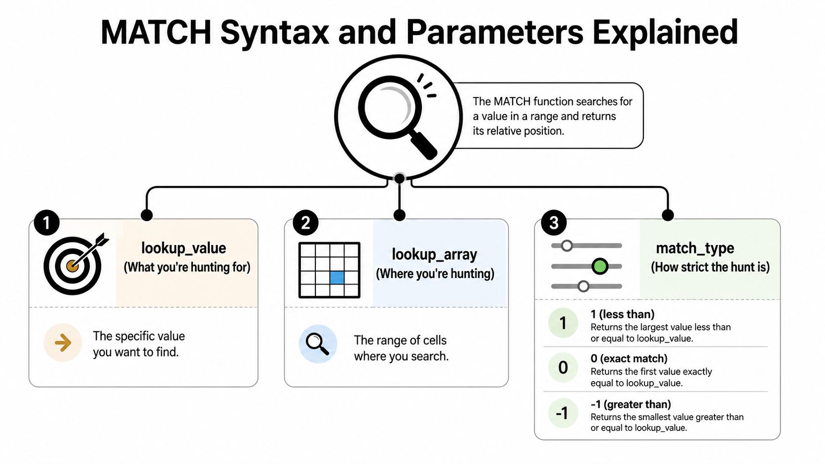
The core syntax is simple: =MATCH(lookup_value, lookup_array, [match_type]) (Microsoft Support). Think of it as three questions in a row, what are you searching for, where are you searching, and how exact should the search be? Once you separate those parts, the formula gets a lot less mysterious.

Start with a tiny example. Put 5, 25, and 38 in cells A1:A3, then type =MATCH(25,A1:A3,0). Excel returns 2 because 25 is the second item in that range (Microsoft Support).

Here's the part that trips people up most often. MATCH works with either a single row or a single column, not a whole table, so your lookup range needs to be a simple line of cells, not a block (GeeksforGeeks). That design is why the function feels lean, but also why people sometimes feed it the wrong shape and wonder why the result looks off.

Break the formula into the three pieces

• lookup_value is the thing you want to find.
• lookup_array is the row or column where Excel should search.
• match_type tells Excel whether you want an exact hit or a sorted approximate result.

The moment of confusion usually happens at match_type. If you choose the wrong one, the formula can look valid and still give you the wrong answer.

The safest habit is to type the exact lookup first, then choose the search range, then decide whether you want strict matching or a sorted search. That order keeps you from guessing at the end and changing the wrong argument when the result looks strange.

Exact vs Approximate Matching and Why Sort Order Matters

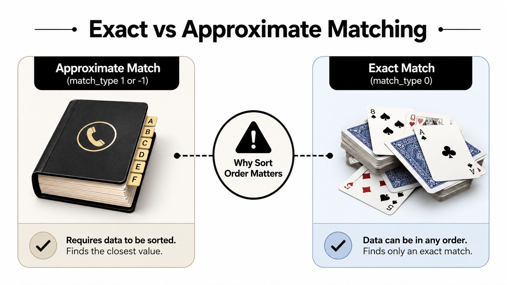
Many learners slip here because 0, 1, and -1 sound like tiny variations but behave very differently. Microsoft and common Excel references describe 0 as an exact match, 1 as an approximate match in ascending order, and -1 as an approximate match in descending order, with 1 as the default if you leave match_type out (Microsoft Learn video). That default catches people off guard all the time.

A phone book is sorted, a shuffled deck of cards isn't. Approximate matching depends on order because Excel is trying to decide what the closest valid item is, so it needs the data arranged in a way that makes that decision meaningful. Exact matching doesn't rely on sort order, because Excel is only looking for one precise value.

Use the right match type for the job

• 0 for exact match. Use this when you want the item only if it matches exactly, like a product code or an ID.
• 1 for ascending approximate match. Use this on sorted low-to-high data when you want the exact value or the next largest item, depending on the dataset's structure.
• -1 for descending approximate match. Use this on sorted high-to-low data when you want the exact value or the next smallest item.

If you forget the sort requirement, the formula may still return something, which is worse than a clean error. A wrong-looking answer in a worksheet can hide for a long time, especially when the cells around it seem fine. That's why many Excel users treat approximate MATCH like a specialist tool, not a default habit.

Practical rule: If the list isn't sorted the way the match type expects, use 0 or sort the list first.

The safe mental model is simple. Exact match asks, “Is this item here?” Approximate match asks, “Given the order of this list, what's the closest valid stop?”

Wildcards, Case Sensitivity, and Practical MATCH Examples

MATCH is forgiving about letter case, so if you search text, Excel doesn't care whether your lookup starts with uppercase or lowercase letters (GeeksforGeeks). That removes one common fear right away. You don't need to build separate formulas for jo and Jo.

Wildcards are the other useful trick. ? stands for a single character, and * stands for any sequence of characters, so a lookup like MATCH("Jo*", names, 0) can find the first name that starts with Jo when you're using text entries. That makes MATCH handy in lists where the beginning of the text matters more than the full string.

MATCH Wildcard Cheat Sheet

A product catalog is a good place to use this. If the item names vary slightly but share a clear prefix, a wildcard lookup can narrow the search without you manually filtering the list first. A roster works the same way when you're trying to find the first name that fits a pattern rather than an exact full-text match.

The other strength is that MATCH can give you a row or column position that feeds another formula. That matters when the value you want lives somewhere else in the sheet and you don't want to hard-code its address. You can search one list, get the index, and hand that index to a second formula that retrieves the linked data.

Here's the useful pattern to remember. Text search is case-insensitive, wildcards broaden your options, and the function still returns a position, not the matched text itself. That makes it a clean fit for lookup chains where another formula does the actual retrieval.

Combining MATCH with INDEX and a Look at XMATCH

MATCH becomes much more useful when you let INDEX do the grabbing. MATCH finds the position, then INDEX uses that position to return the actual value from another row or column. That two-step setup is why the pair shows up so often in lookup formulas, and it's also why people use it when they want more flexibility than a basic VLOOKUP-style pattern offers.

A simple way to think about it is this. MATCH points to the seat, INDEX hands you the person sitting there. Once that clicks, left lookups make more sense too, because you're no longer limited to “find something in the first column and return something to the right.”

The classic benefit is column flexibility. If columns get rearranged, a MATCH-based setup is usually easier to maintain because the position can be found dynamically instead of being tied to a fixed column number. That's one reason many learners move from VLOOKUP habits to INDEX and MATCH patterns.

For a practical workflow angle, you can also connect lookup logic with Google Ads match type management in Sheets when your data work spills into campaign cleanup. That kind of job often needs position-based logic more than a rigid table scan.

The modern alternative you should know

XMATCH is the newer lookup cousin many users learn after MATCH. It's designed as a more modern search tool, and it gives you a cleaner path when you're building newer workbooks or want lookup behavior that's easier to read at a glance. If MATCH feels like the classic mechanic's wrench, XMATCH is the updated version many people reach for once they know what they need.

Practical rule: Use MATCH when you want the position. Use INDEX when you want the value. Learn XMATCH when you want the newer lookup style.

The classic two-way pattern is INDEX with two MATCH functions, one for the row and one for the column. That setup is especially useful when you're pulling from a grid and need Excel to find both coordinates before returning the final result.

Common MATCH Errors and How to Fix Them Fast

The most common failure mode is #N/A. That usually means Excel couldn't find the value, or the match_type doesn't fit the data you gave it. The fastest fix is to confirm the lookup value really exists and then check whether you should be using 0 instead of an approximate match setting.

#VALUE! tends to show up when the lookup range isn't shaped the way MATCH expects, or when the data types don't line up cleanly. If you're feeding text into a number search, or a block of cells into a function that wants a single row or column, the result can break. Normalizing the data and simplifying the range usually clears it up.

Hidden spaces cause quieter pain. A value that looks identical to the eye may not match because there's an extra space before or after the text, so Excel treats it like a different entry.

Quick troubleshooting checklist

• Check the data shape. MATCH wants a single row or single column.
• Check the sort order. Approximate matches need sorted data in the right direction.
• Check the text itself. Extra spaces can block a match that looks obvious.
• Check the match type. If you want an exact hit, use 0.

The sneakiest bug is the wrong approximate match on unsorted data. Excel may return a result without warning, and that result can look believable enough to slip into a report. That's why a lot of experienced users treat 0 as the safe starting point unless they have a clear reason to use 1 or -1.

If the answer looks almost right, don't trust it yet. Confirm the sort order before you trust an approximate match.

Performance Tips and Real-World Use Cases

MATCH works best in workbooks where the formula needs a position, not the final answer. A dropdown-driven dashboard can use MATCH to find the chosen region, then pass that position to INDEX so the report updates from the correct row. Tiered pricing sheets use the same logic when the lookup needs to land in the right bracket instead of grabbing the first similar value it sees.

Sort order decides whether MATCH behaves like a careful librarian or a rushed file clerk. With 0, MATCH looks for an exact item and does not care whether the list is sorted. With 1 or -1, the list has to be sorted the right way, because Excel is using the order of the data to decide which position counts as the match. If that sounds easy to mix up, it usually is. The mistake happens when someone treats an approximate match like a search for any visible item, then assumes the formula will correct the data order for them.

A 10,000-row pricing table can expose this difference fast. If every change forces a large range to recalculate, the workbook can start to feel sluggish, especially when MATCH is chained into several other formulas. Keeping the lookup range tight helps more than many learners expect, because Excel has less data to scan each time it recalculates. Volatile functions in the same workbook can make that slower, so a cleaner lookup design usually pays off in day-to-day use. Newer builds can also use XMATCH, which reads more clearly and fits better in formulas that need a more modern lookup style.

MATCH also fits well into workflows that mix spreadsheet logic with external data. A practical example is connecting Google Ads data to Google Sheets, where MATCH can help line up keywords, regions, or campaign labels before other formulas pull in the final values. Tools like Keywordme can also help teams manage match-type decisions in Google Ads keyword work without turning each adjustment into manual copy-paste.

One useful rule is to reserve MATCH for finding positions in a list. INDEX then uses that position to return the value you want, and XMATCH can replace older setups when you want clearer lookup logic. The big performance win is to avoid running MATCH across oversized ranges when only a small slice of the table matters.

If you keep that model in mind, the formula stops feeling like syntax trivia and starts acting like a reliable lookup tool. That is the point where MATCH becomes a habit you can trust in dashboards, pricing sheets, and keyword workflows.